1 Introduction
Deep learning compilers rely heavily on manual written templates to schedule computations of deep learning kernels. Leveraging polyhedral models, the scheduling can be done automatically. The polyhedral model is a powerful abstraction for compiler optimization, turning scheduling problems into integer linear programs (ILPs). However, these ILPs may not be solvable due to scalability issues.
2 Outline
- Started project: Deep learning compiler studies
- Read a paper: Leveraging the polyhedral model in deep learning compilers may be a good research direction
- Read another paper: Solving ILPs using neural networks
- Simple idea: Leverage neural network in the ILP solving process of the polyhedral scheduler inside the deep learning compiler
- Investigated if the polyhedral scheduler’s internal solver could be replaced: No.
- Investigated the internal solver and learned about the PIP algorithm.
- Learned about the formulation of ILPs
- The PIP algorithm seemed good enough in most cases under current settings, perhaps we should consider another way of formulating ILPs
- Or we could invent some neural network model tuned for ILPs in polyhedral compiling
3 Background
3.1 Deep learning compilers
Deep learning frameworks like TensorFlow and Pytorch express deep neural networks as directed acyclic graphs of tensor operations. These frameworks provide promising performance for many applications by leveraging highly optimized vendor libraries and making transparent use of architectures, but fall short in supporting custom operators invented by users/high-level optimizing engines, exploiting transformations across operators, and tuning for divergent sizes and shapes.
Deep learning compilers like TVM, Tensor Comprehensions and Tiramisu have been devised to address these challenges, bridging the gap between custom operators and diverse architectures.
3.2 Polyhedral scheduling
The polyhedral model is capable of a statement-wise representation of a program. Manipulation on top of the polyhedral model is convenient, in the form of affine transformations.
4 Exploration
To further examine the problem, we explored the following topics:
4.1 Formulating the scheduling problem as an ILP
We mainly looked into the Pluto algorithm, the main scheduling algorithm used in the ISL, a popular polyhedral scheduling library. We discuss here how the variables, objective and constraints of the ILP are constructed.
Variables
- Transformation coefficients: They directly specify the transformation.
- Other auxiliary variables: Including variables denoting upper bounds of dependency distances.
Objective
There are several objectives and the problem is actually described as a multi-objective (or lexicographical minimal to be precise) ILP problem. However, we believe the primary objective is to minimize dependency distances between program statements.
Constraints
- Validity schedule constraints: Ensures that dependencies do not get corrupted after transformation i.e., for the data dependency $a \rarr b$, constrain that after transformation $a' \rarr b'$.
- Proximity schedule constraints: Denotes upper bounds of dependency distances.
- Coincidence schedule constraints: Specifies an instance be executed together with another, i.e. parallelism.
4.2 Solving an ILP by the modified cutting-plane method
This is the default algorithm used by the ISL polyhedral library, namely Feautrier’s Parametric Integer Programming. It is based on the dual simplex method. Gomory cuts are applied to give integral solutions. Through elaborate manipulation of the simplex tableau, lexicographical minimal solutions can be found. We think this is extraordinary because the lexicographical minimal problem format differed so much from the canonical form yet the algorithm is only a few tweaks away from the classic cutting-plane method.
Lexicographical minimum objective
Denote $(x_1, x_2, …, x_n) < (y_1, y_2, …, y_n)$ iff. $x_i = y_i, 1 \le i \le k < n$ and $x_{k+1} < y_{k+1}$.
In a lexicographical minimal ILP problem with variables $x_1, x_2, …, x_n$, instead of having an objective in the form of $\min{(a_1x_1+a_2x_2+…+a_nx_n)}$, the objective is something like $\min{(x_1,x_2, …, x_k)}$. It is like a simple form of multi-objective ILP, with each objective being a variable. However, off-the-shelf ILP solvers are not good at solving multi-objective ILP problems.
4.3 Solving an ILP by neural networks
In the paper Solving Mixed Integer Programs Using Neural Networks, Google proposed a method for solving ILPs using neural networks.
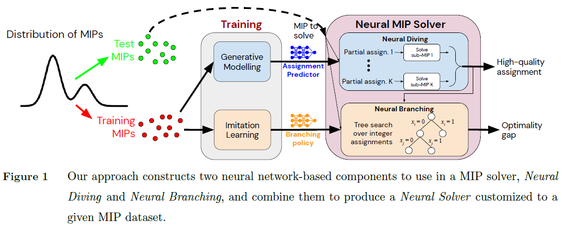
The neural solver has two neural network-based components. Combining them gives great results (faster to optimal or more accurate solutions under given time) on real-world large-scale datasets.
Neural Diving: Uses a generative neural network model to predict high-quality partial variable assignments, effectively pruning the search space and accelerating the solving process.
Neural Branching: Uses neural networks to imitate the Full Strong Branching (FSB) expert policy. The FSB policy generally generates smaller search trees in branch-and-bound, with the cost of heavy computation. Neural Branching can achieve similar effects with much faster neural network-based predictions in place of the heavy brutal computation.